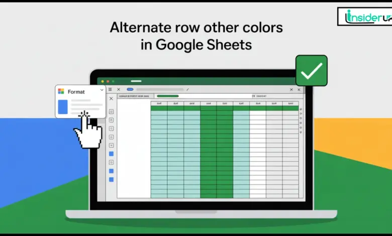
If you’ve ever opened a spreadsheet and found your eyes blurring as you try to follow a row across dozens of columns, you’re not alone. Google Sheets is a fantastic tool for organizing data, but as your tables grow, keeping them readable becomes a real challenge. One of my favorite tricks to make data pop and stay organized? Coloring every other row! In this guide, I’ll walk you through everything you need to know about how to color every other row in Google Sheets—with easy steps, real-world examples, and some handy advanced tips.
Let’s face it—Google Sheets is everywhere. From small businesses to classrooms, it’s the go-to for organizing everything from sales data to soccer schedules. But as your data grows, so does the challenge of keeping it readable. That’s where coloring every other row comes in. This simple formatting trick, also called “zebra striping,” makes your tables easier to read and way more professional. In this guide, I’ll show you all the ways to do it, whether you’re a newbie or a spreadsheet pro.
Also Read:
Why Is My PC Taking a Long Time to Shut Down?
How Do I Flip a Picture in PowerPoint
Can Your Password Protect a Folder on Mac?
Vlc Player How to Rotate Video
What Can I Use Instead of Facebook?
Why Color Every Other Row in Google Sheets?
Before we get into the “how,” let’s talk about the “why.” Why bother with alternating row colors in the first place?
- Improved Readability: Alternating colors make it easier to track data across rows, especially in wide tables.
- Visual Appeal: Your spreadsheets look cleaner, more organized, and more professional.
- Error Reduction: It’s easier to spot mistakes or mismatched data when your eyes aren’t struggling to follow a single line.
- Professional Presentation: Whether you’re sharing a budget report or a project tracker, a well-formatted sheet makes a great impression.
- Common Use Cases: Financial reports, attendance lists, inventory trackers, and more all benefit from this simple formatting.
Methods to Color Every Other Row
There are several ways to color every other row in Google Sheets. Let’s break down the most popular methods, so you can pick the one that fits your needs.
Using Built-in Alternating Colors Feature
This is by far the easiest and quickest way to apply alternating row colors.
Step-by-Step Guide
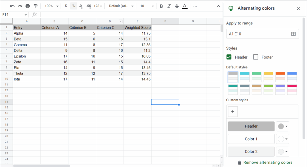
- Select Your Data Range: Click and drag to highlight the area you want to format.
- Go to the Menu: Click on
Formatin the top menu. - Choose Alternating Colors: Select
Alternating colorsfrom the dropdown. - Customize Your Style: A sidebar will appear. You can choose from preset color styles or create your own.
- Apply and Done: Click
Doneto apply the formatting.
Example Table
| Step | Action | Where to Click |
|---|---|---|
| 1 | Select your data range | Click and drag |
| 2 | Open Format menu | Format > |
| 3 | Choose Alternating Colors | Alternating colors |
| 4 | Pick a color style | Sidebar |
| 5 | Apply | Done |
Customizing Colors
You can personalize the header, even and odd row colors. This is perfect for matching your company’s branding or just making your sheet look the way you want.
Tip: If you add more rows, Google Sheets automatically applies the alternating color pattern to the new data!
Using Conditional Formatting
If you want more control or need to color every nth row (not just every other one), Conditional Formatting is your friend.
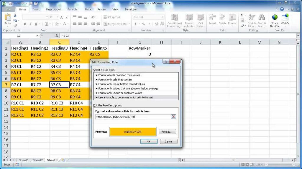
What is Conditional Formatting?
Conditional Formatting lets you set up rules that automatically change the appearance of cells based on their content or position.
Step-by-Step Guide
- Select Your Data Range: Highlight the rows and columns you want to format.
- Open Conditional Formatting: Go to
Format>Conditional formatting. - Set Up the Rule:
- In the sidebar, under “Format cells if,” choose “Custom formula is.”
- Enter the formula: text
=ISEVEN(ROW())This formula colors every even-numbered row. To color odd rows, use=ISODD(ROW()).
- Choose Your Formatting Style: Pick your background color.
- Click Done: The formatting will apply instantly.
Example Table
| Formula Used | Effect |
|---|---|
| =ISEVEN(ROW()) | Colors even-numbered rows |
| =ISODD(ROW()) | Colors odd-numbered rows |
| =MOD(ROW(),3)=0 | Colors every third row |
Why Use Conditional Formatting?
- More flexibility (color every nth row, combine with other rules)
- Works on any range, not just full rows
- Can be used alongside other formatting rules
Manual Row Coloring
Sometimes, you just want to color a few rows by hand—maybe for a small table or a one-off highlight.
When to Use Manual Coloring
- Small tables where automation isn’t needed
- Highlighting specific rows for emphasis
How to Do It
- Select the Row(s): Click the row number(s) on the left.
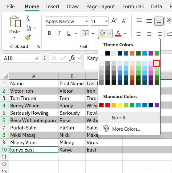
- Open Fill Color: Click the paint bucket icon in the toolbar.
- Pick Your Color: Choose the background color you want.
Pros and Cons
| Pros | Cons |
|---|---|
| Quick for small tables | Tedious for large tables |
| Full control | Not dynamic (new rows not colored) |
Advanced Tips and Customization
Once you’ve mastered the basics, you can take your formatting to the next level!
Custom Color Schemes and Branding
- Use your brand’s colors for headers and rows.
- Save custom styles for consistency across multiple sheets.
Applying Alternating Colors to Dynamic Ranges
- With Alternating Colors, new rows are colored automatically.
- With Conditional Formatting, make sure your range covers future data.
Coloring Every Nth Row
Want to color every third or fourth row? Use a custom formula in Conditional Formatting:
text=MOD(ROW(),3)=0 // Colors every third row
Combining with Other Formatting Rules
- Highlight duplicates
- Color cells based on value
- Apply bold or italic formatting to specific rows
Troubleshooting
Here are some common issues and how to fix them:
Common Issues
| Issue | Solution |
|---|---|
| Colors not applying to new rows | Expand your formatting range or use Alternating Colors |
| Formatting disappears | Check if another rule is overriding it |
| Need to remove alternating colors | Select range, go to Format > Alternating colors, click Remove |
How to Remove Alternating Colors
- Select the colored range.
- Go to
Format>Alternating colors. - Click
Remove alternating colors.
Applying Formatting to New Data Automatically
- Use Alternating Colors for automatic updates.
- With Conditional Formatting, set your range to include potential new rows.
Google Sheets Color Every Other Row on Mobile
You can also format rows on your phone or tablet using the Google Sheets app for Android or iOS.
Steps for Mobile Devices
- Open Your Sheet: Launch the Google Sheets app.
- Select Your Range: Tap and drag to highlight cells.
- Tap Format: Look for the paint roller icon.
- Choose Alternating Colors: If available, select it and pick your style.
Limitations and Workarounds
- Some advanced formatting options (like custom formulas) are only available on desktop.
- For more complex needs, format your sheet on a computer and view it on mobile.
Use Cases and Real-World Examples
Let’s see how alternating row colors can make a difference in real-world spreadsheets.
Example 1: Financial Spreadsheet
| Month | Income | Expenses | Profit |
|---|---|---|---|
| January | $5,000 | $3,200 | $1,800 |
| February | $4,800 | $2,900 | $1,900 |
| March | $5,200 | $3,100 | $2,100 |
With alternating colors, it’s much easier to follow each row across columns.
Example 2: Attendance Tracker
| Name | Present | Absent |
|---|---|---|
| Alice Smith | 20 | 2 |
| Bob Jones | 19 | 3 |
| Carol Lee | 21 | 1 |
Example 3: Inventory List
| Item | Quantity | Location |
|---|---|---|
| Laptops | 15 | Room 101 |
| Projectors | 5 | Room 102 |
| Whiteboards | 8 | Room 103 |
Best Practices for Spreadsheet Design
A well-designed spreadsheet is more than just pretty colors. Here are some tips:
- Consistency: Use the same color scheme throughout your document.
- Accessibility: Choose high-contrast colors for better visibility, especially for users with color blindness.
- Clarity: Avoid too many colors or distracting patterns.
- Simplicity: Less is often more—use colors to enhance, not overwhelm.
Integrating with Google Apps Script
For power users, Google Apps Script lets you automate alternating row colors and more.
Sample Script: Color Every Other Row
javascriptfunction colorAlternateRows() {
  var sheet = SpreadsheetApp.getActiveSpreadsheet().getActiveSheet();
  var range = sheet.getDataRange();
  var rows = range.getNumRows();
  var cols = range.getNumColumns();
  var bgColors = [];
  for (var i = 1; i <= rows; i++) {
    var rowColor = (i % 2 == 0) ? "#f2f2f2" : "#ffffff";
    var row = [];
    for (var j = 1; j <= cols; j++) {
      row.push(rowColor);
    }
    bgColors.push(row);
  }
  range.setBackgrounds(bgColors);
}
How to Use
- Open your sheet.
- Go to
Extensions>Apps Script. - Paste the code and save.
- Run the function.
When to Use Scripting
- Automate formatting for large or frequently updated sheets
- Apply custom logic beyond built-in features
Conclusion
Coloring every other row in Google Sheets is a simple but powerful way to make your data easier to read, more attractive, and more professional. Whether you use the built-in Alternating Colors feature, Conditional Formatting, or even Google Apps Script, you have all the tools you need to create beautiful, functional spreadsheets.
So go ahead—try it out on your next project! Your eyes (and your colleagues) will thank you.
Frequently Asked Questions
1. How do I quickly color every other row in Google Sheets?
The fastest way is to use the built-in Alternating Colors feature. Select your data range, go to the Format menu, choose Alternating colors, and pick your desired color scheme. Click Done, and Google Sheets will automatically apply the pattern.
2. Can I customize the colors used for alternating rows?
Yes! In the Alternating Colors sidebar, you can select custom colors for the header, odd rows, and even rows. You can also save your preferred scheme as a custom style for future use.
3. What if I want to color every third or fourth row, not just every other row?
Use Conditional Formatting with a custom formula. For every third row, use =MOD(ROW(),3)=0 as your formula. Adjust the number to match the interval you want (e.g., =MOD(ROW(),4)=0 for every fourth row).
4. How do I use conditional formatting to alternate row colors?
- Select your range.
- Go to
Format>Conditional formatting. - Under “Format cells if,” choose “Custom formula is.”
- Enter
=ISEVEN(ROW())for even rows or=ISODD(ROW())for odd rows. - Set your color and click
Done.
5. Will alternating colors update automatically when I add new rows?
If you use the Alternating Colors feature, new rows added within the formatted range will be colored automatically. With Conditional Formatting, make sure your rule covers the full (and future) data range to ensure new rows get formatted.